The 2022 Treasury curve: rising yields, a changing spread
A frozen historical case study separates the level of yields from the shape of the curve.
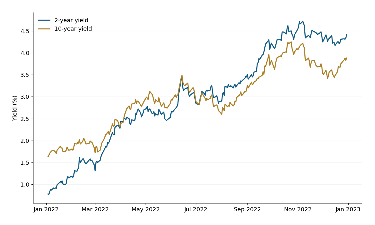
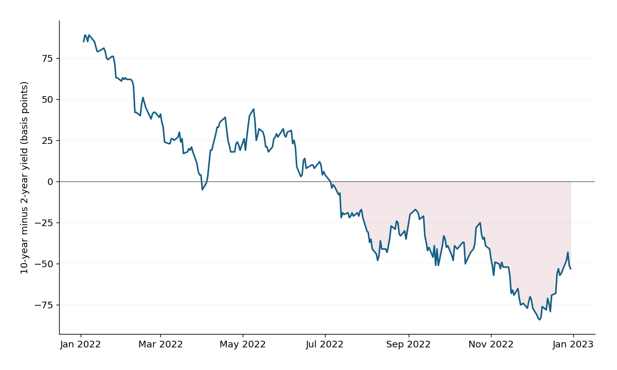
Across 249 matched observations in 2022, the 10-year minus 2-year spread moved from 85 basis points on 2022-01-03 to -53 on 2022-12-30. The spread was negative on 125 observed dates. These are retrospective yield observations, not investment returns or a trading test.
The question and the fixed window
Can a broad rise in yields coexist with a curve that moves from positively sloped to inverted? This study answers that descriptive question for the calendar year 2022. The period is chosen as a known policy-tightening episode, not presented as a randomly selected validation sample. Its usefulness is the distinction between rate level and curve shape. It cannot establish how often inversion forecasts an event or identify a profitable strategy.
The calculation uses daily constant-maturity Treasury yields at two years and ten years. These are estimated yields for specified maturities rather than prices of two securities held continuously for a year. A bond investor also receives income and experiences changes in maturity, duration and the bond selected. Subtracting two yield series does not produce that investor's holding-period return.
Source, retrieval and observation alignment
The source is the Federal Reserve Board H.15 release as distributed by FRED, using series DGS2 and DGS10. Both series are quoted in percent and are not seasonally adjusted. The downloadable source extracts and the transformed table are retained with this publication. The machine-readable record includes retrieval times, source URLs and SHA-256 digests so the release can be checked against its actual inputs.
Only dates with a numeric value in both series enter the paired table. Missing observations are omitted; there is no forward fill, interpolation or replacement with zero. The resulting 249 observations are matched daily records, not 365 calendar-day measurements. The study uses the data retrieved for this release, not an ALFRED reconstruction of information available on each historical date. That distinction matters for any later decision-timing experiment.
Reproduce the arithmetic
For each matched date, subtract the two-year yield from the ten-year yield. Because the source values are percentages, multiply that difference by 100 to express it in basis points. The published CSV retains the two input levels beside the computed spread. A reader can therefore verify an individual row without needing a proprietary model or an account.
On the first observed date, 1.63% minus 0.78% equals 0.85 percentage points, or 85 basis points. On the final observed date, 3.88% minus 4.41% equals -0.53 percentage points, or -53 basis points. Both yields are higher at the end than at the start, yet the spread is lower because the shorter yield rose by more. The endpoint comparison is descriptive and omits the path between those dates.
| Observation | 2-year yield | 10-year yield | 10y - 2y spread |
|---|---|---|---|
| 2022-01-03 | 0.78% | 1.63% | 85 bp |
| 2022-12-07 | 4.26% | 3.42% | -84 bp |
| 2022-12-30 | 4.41% | 3.88% | -53 bp |
What the path adds
The lowest observed spread in this extract is -84 basis points on 2022-12-07. A simple count finds 125 matched dates with a strictly negative spread; a zero spread would not count as inversion under this definition. This count describes the selected sample only. It is not the number of calendar days in an uninterrupted inversion and does not measure the probability of recession.
Plotting both yield levels and their difference prevents a common reading error. The level chart shows the common direction over much of the window. The spread chart isolates relative movement. Looking only at one can hide the other. An investment thesis should specify whether it concerns outright rate exposure, relative maturity exposure or a macro interpretation before choosing a chart as evidence.
From observation to a research question
An inverted curve can motivate research on expected policy rates, term premia, growth expectations and funding conditions. Those explanations are not identified by this two-series chart alone. The same observed spread may reflect several forces, and market prices already embed expectations. A defensible next study would state the economic hypothesis, choose additional series, define their availability and freeze the evaluation window before looking at the result.
A portfolio application needs another layer of work. A duration exposure responds to changes in the relevant yield curve, while a curve trade has sizing, financing and instrument-selection choices. Neither follows automatically from the fact that the curve is inverted. The duration calculator on this publication illustrates a fixed-sensitivity price approximation; it does not turn this historical chart into a strategy backtest.
Revision record and limitations
This is the first published version, dated 15 October 2026. Its 2022 source snapshot is frozen in the release. A future correction should preserve this version and explain which source row, transformation or interpretation changed. The archive date is the publication date, not a claim that the analysis was written before the historical events unfolded.
The study deliberately uses one country, two maturities and one year. It omits bond income, market execution, transaction costs, credit risk, foreign-exchange translation and other asset returns. It therefore supports a narrow conclusion about yield level versus curve shape. Broader cross-asset conclusions require additional evidence and an explicit design for matching observation times and instruments.
What to retain
- Level and slope are different measures of a yield curve.
- The published spread is reproducible from the matched input rows.
- A descriptive historical chart does not establish a forecast or an executable return.
Source notes
Related research
Interpreting Yield-Curve Shapes and Changes
Describe curve levels, slopes, forwards, and term premiums without treating inversion or steepening as a complete economic forecast.
Duration and the Mechanics of Rate Shocks
Calculate bond-price sensitivity, convexity, and curve exposure while keeping approximations separate from realized returns.
Missing data and market calendars in cross-asset studies
Handle closures, unavailable releases, stale quotes, and asynchronous observations without manufacturing zero returns or future information.
Version 1, 15 October 2026. First publication. Illustrative calculations are identified in context; source observations retain their stated dates.